2 Bayesian Optimization & Gaussian Processes
This post is a brief overview about Bayesian Optimization. We often see this technique used for hyperparameter tuning (like finding the perfect learning rate for a neural net) or in robotics (finding control parameters that maximize walking speed).
The core problem is: How do we optimize a function \(f(x)\) when every evaluation is expensive?
2.1 The Problem Setup
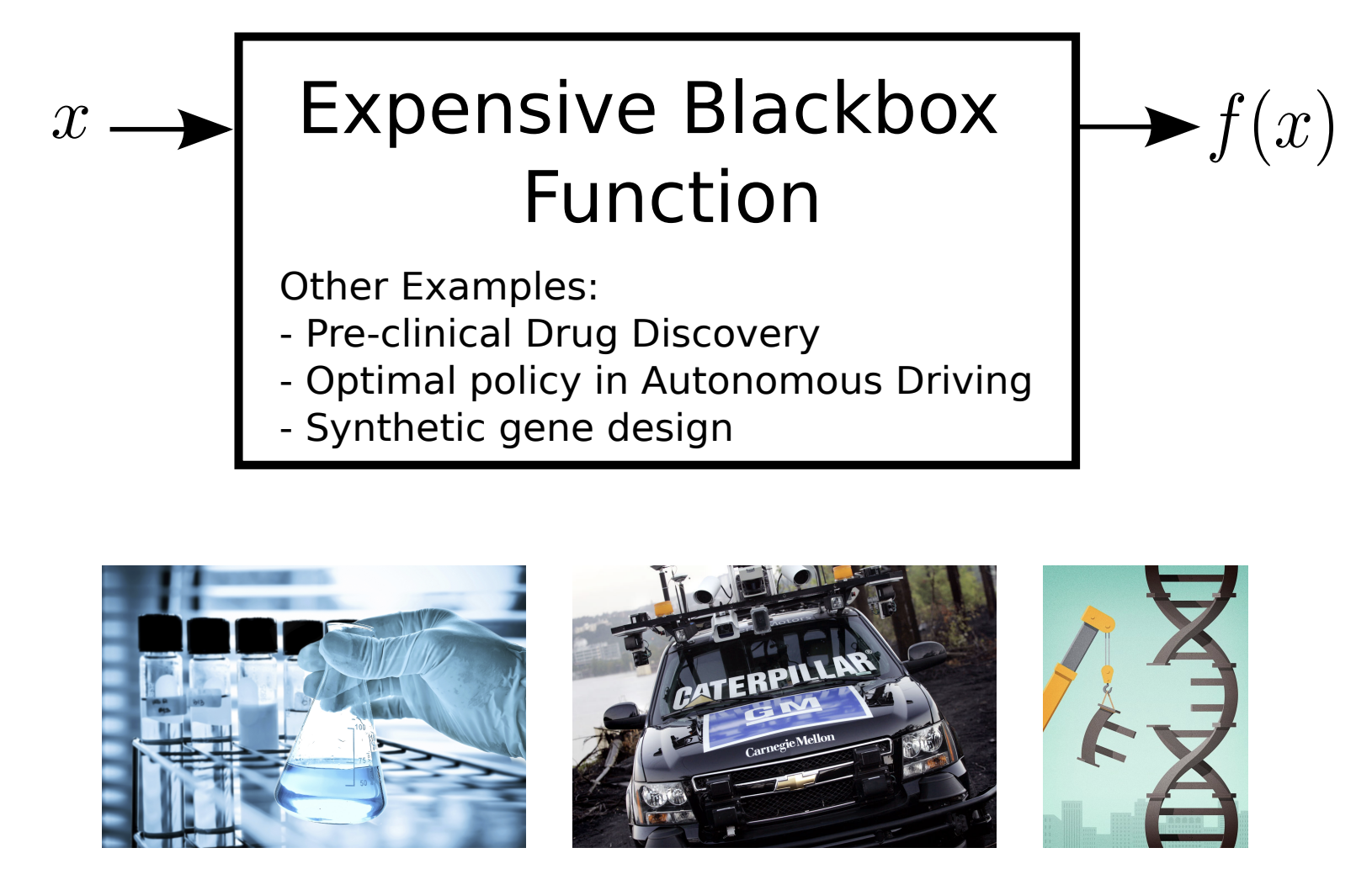
We start with the “Expensive Blackbox Function.” This is the central character of our story. In standard Deep Learning (e.g., SGD), we assume evaluating the gradient is cheap. Here, we assume evaluating \(f(x)\) costs significantly—either time (training a massive model), money (wet lab experiments), or risk (robotics).
The examples given are crucial to understanding why we need this:
- Drug Discovery: We can’t just synthesize random molecules; it takes days in a lab.
- Autonomous Driving: We can’t just try random policies on a highway; a crash is “expensive”.
- Hyperparameter Search: Training a Transformer takes weeks. We can’t grid-search the learning rate.
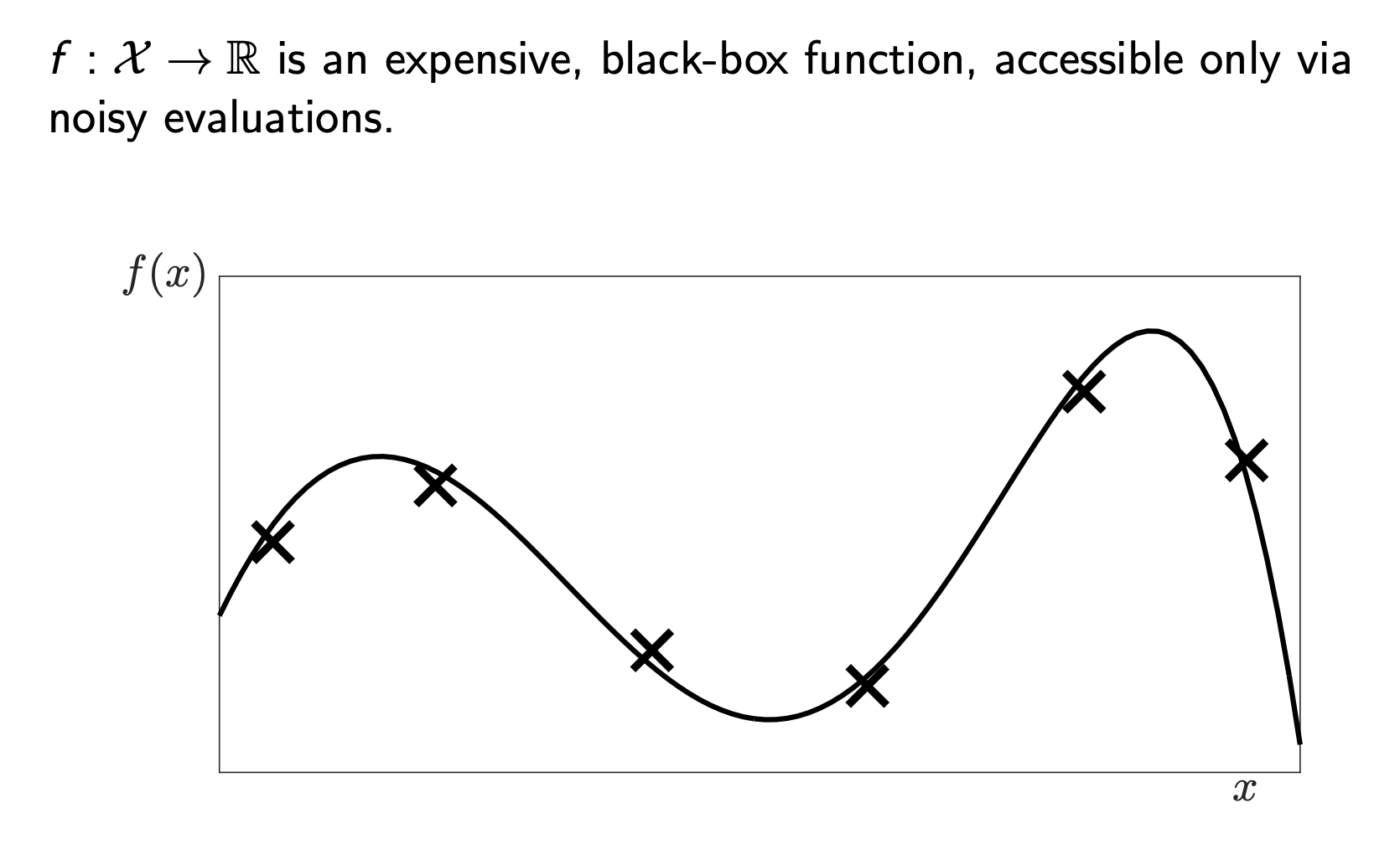
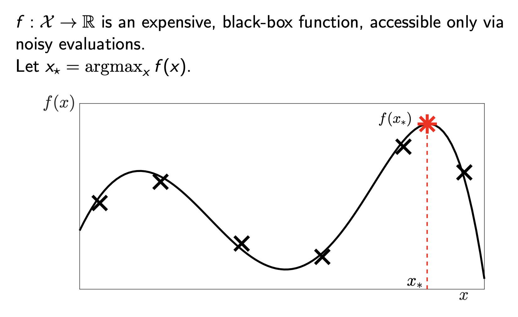
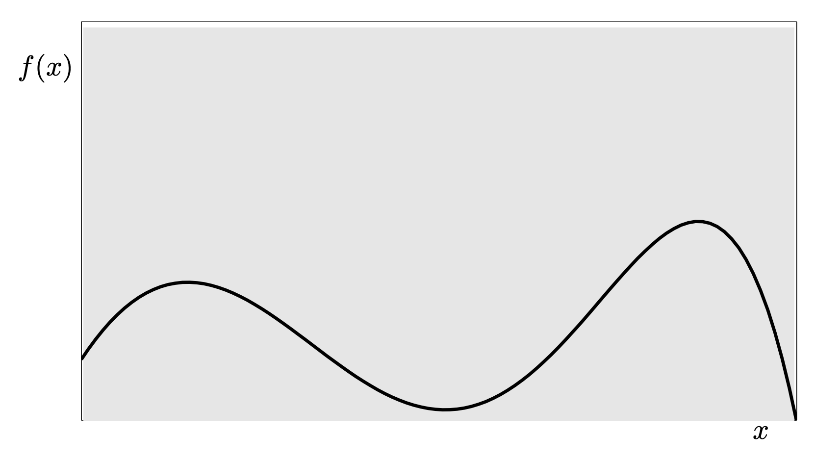
Mathematically, our goal is simply to find \(x_* = \text{argmax}_x f(x)\). However, look at the plot above. We only see the function through “noisy evaluations” (the ‘x’ marks). We don’t know the full curve. We have to guess where the peak (\(x_*\)) is based on limited data.
2.2 The “Brain” - Gaussian Processes
To solve this, we need a model that doesn’t just predict a value, but also tells us how unsure it is. This is where Gaussian Processes (GP) come in.
A GP is a “distribution over functions”.
- Prior: Before we see data, we assume the function is smooth.
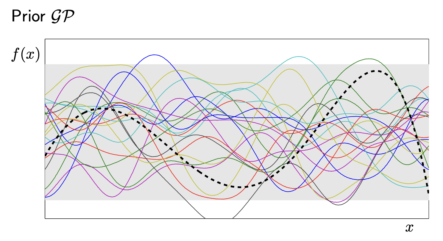
- Posterior: After we see data, we eliminate functions that don’t fit the observations.
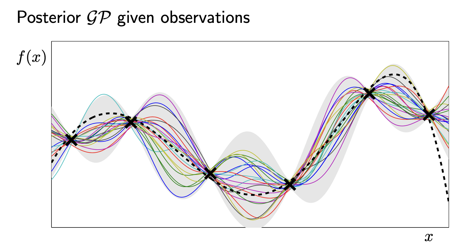
In the image above,
- The Solid Line: The mean prediction \(\mu(x)\). This is what the model thinks the function looks like.
- The Grey Area: The variance \(\sigma^2(x)\). This is the uncertainty.
Notice how the grey area “pinches” at the black crosses? That’s because we know the value there. We are uncertain only in the gaps.
2.2.1 The Math Behind GPs
Formally, a GP is a collection of random variables, any finite number of which have a joint Gaussian distribution. It is fully specified by two things:
- Mean Function \(m(x)\): Usually assumed to be 0 for simplicity.
- Covariance Function \(K(x, x')\) (The Kernel): This defines “similarity.”
The math below shows how we actually compute the posterior.
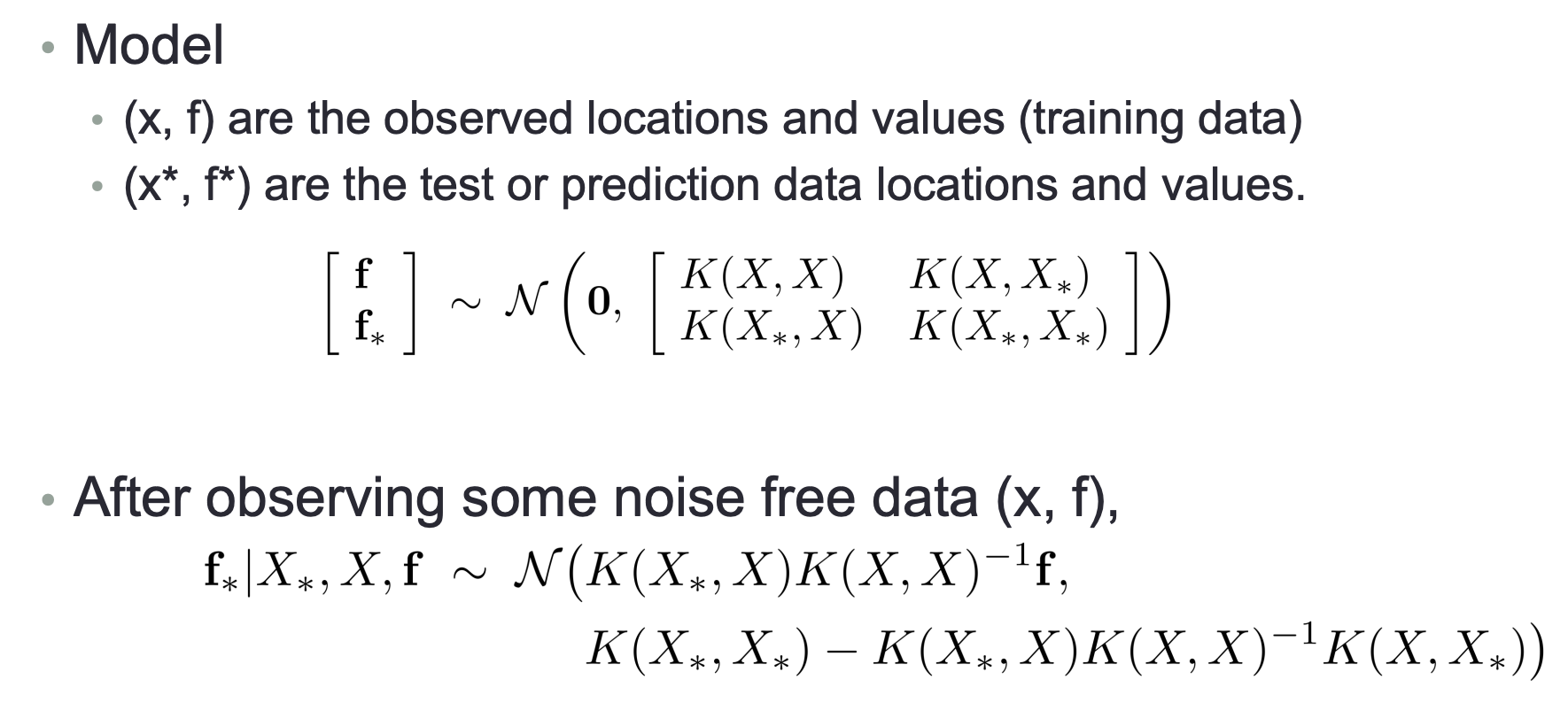
If we have observed data \((X, f)\) and want to predict at a new point \(X_*\), the conditional distribution is:
\[f_* | X_*, X, f \sim \mathcal{N}(\mu_{post}, \Sigma_{post})\]
The formula involves inverting the kernel matrix \(K(X,X)^{-1}\). This inversion is technically \(O(N^3)\), which is why GPs are computationally expensive if you have massive datasets (but perfect for “small data” problems like robot tuning).
2.3 Strategy 1 - GP-UCB
Now that we have a model (the GP), how do we choose the next experiment? We need an Acquisition Function.
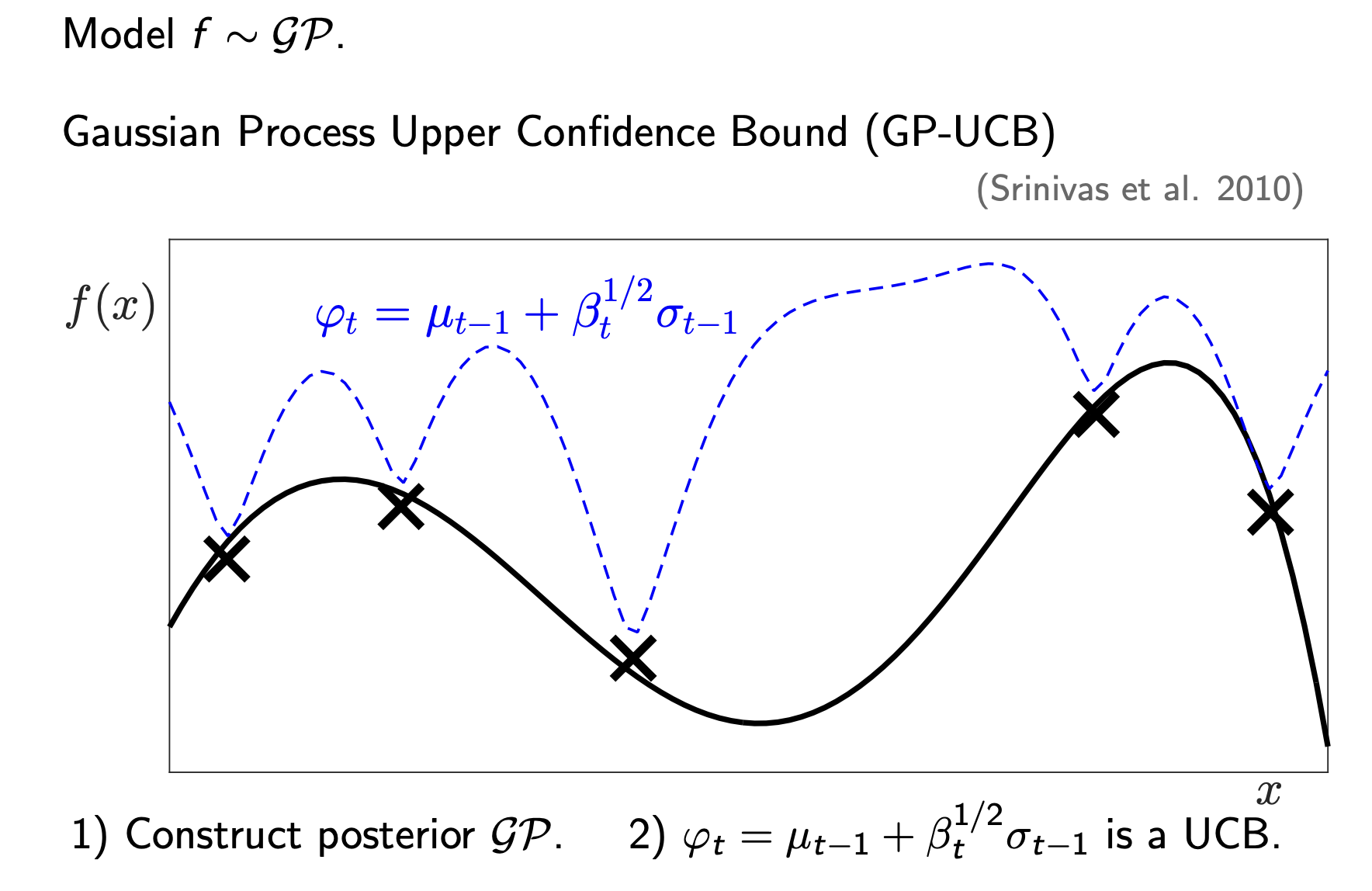
The first strategy is Upper Confidence Bound (UCB) (Srinivas et al. 2010). The intuition is “Optimism in the face of uncertainty”. The formula (from Srinivas et al., 2010) is:
\[\varphi_t(x) = \mu_{t-1}(x) + \sqrt{\beta_t} \cdot \sigma_{t-1}(x)\]
- \(\mu_{t-1}\): Exploitation. Go where the mean is high.
- \(\sigma_{t-1}\): Exploration. Go where we are uncertain (the grey area is wide).
- \(\beta_t\): A parameter that balances the two.
Look at the image above:
- The Black Line is the true function.
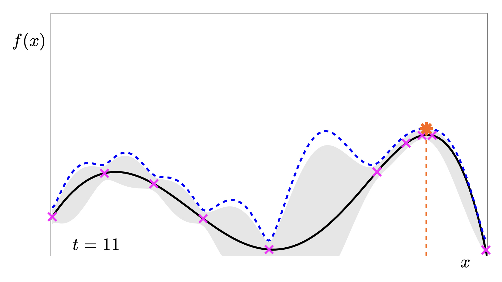
- The Dashed Blue Line is the UCB (\(\varphi_t\)).
- We pick the peak of the dashed blue line (the purple circle) as our next trial.
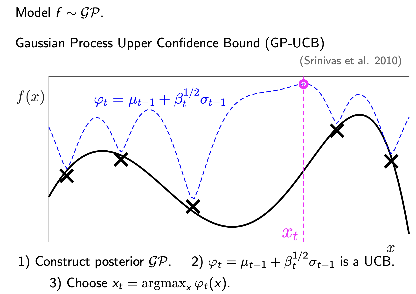
In the next step, because we sampled that peak (the new ‘x’), the uncertainty there has collapsed to 0. The UCB curve (dashed blue) will changes shape, forcing us to look somewhere else next time.
2.3.1 GP-UCB in Action
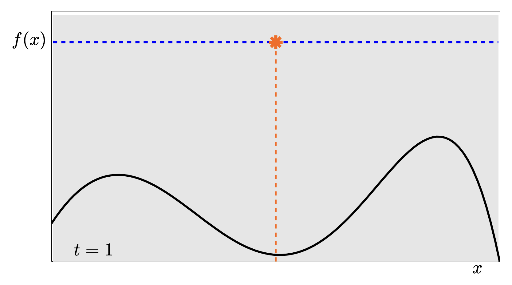

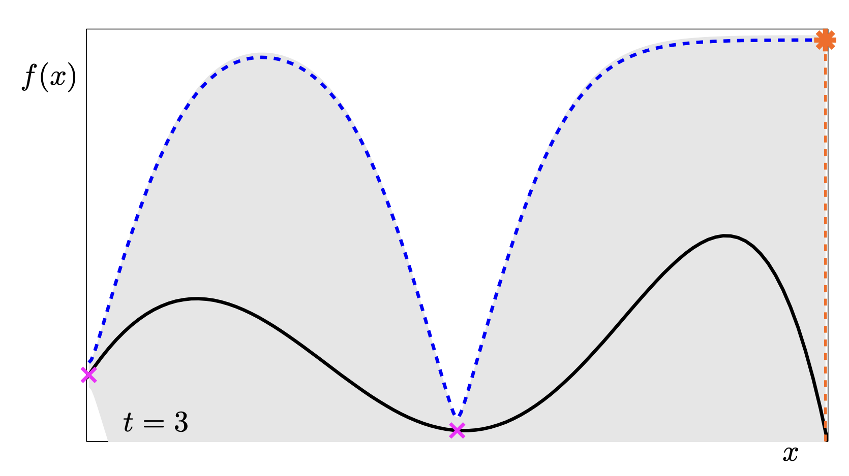
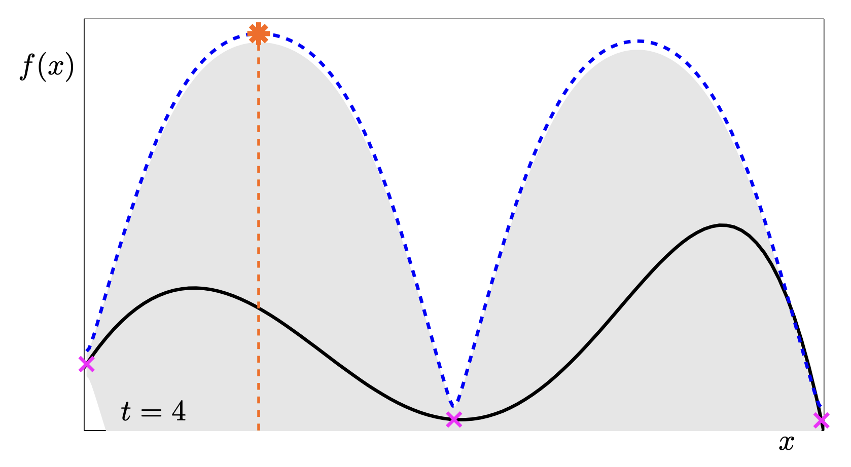
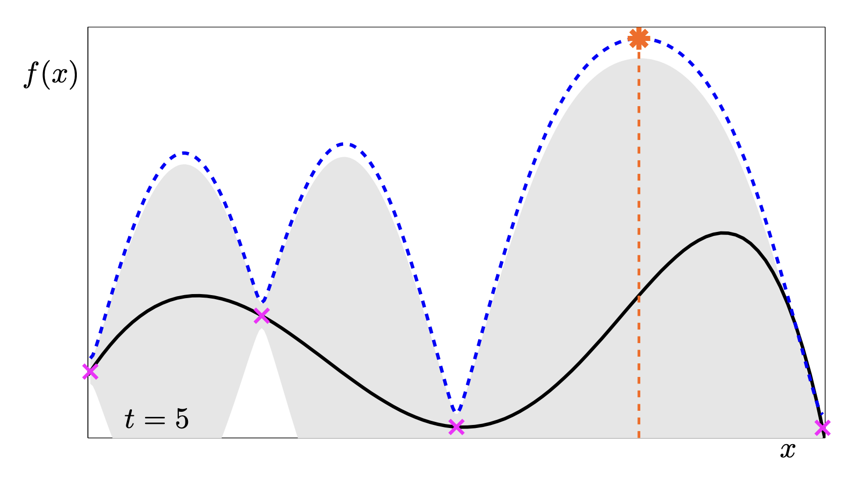
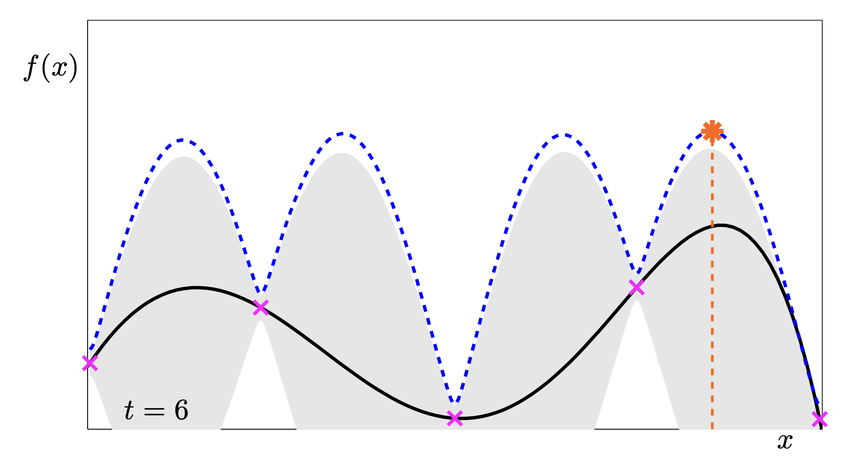
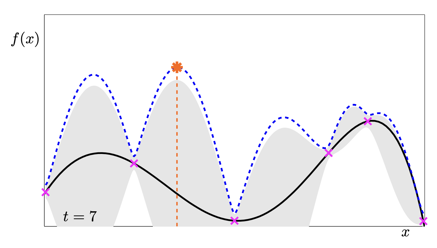
This sequence is a fantastic animation of the convergence.
- t=1: We know almost nothing. We just pick the middle.
- t=2: The uncertainty drops in the middle, pushing the UCB peaks to the far left and right.
- t=5: We have found a “local” maximum on the right, but the UCB is still high on the left, telling us “Hey, you haven’t checked here yet!”.
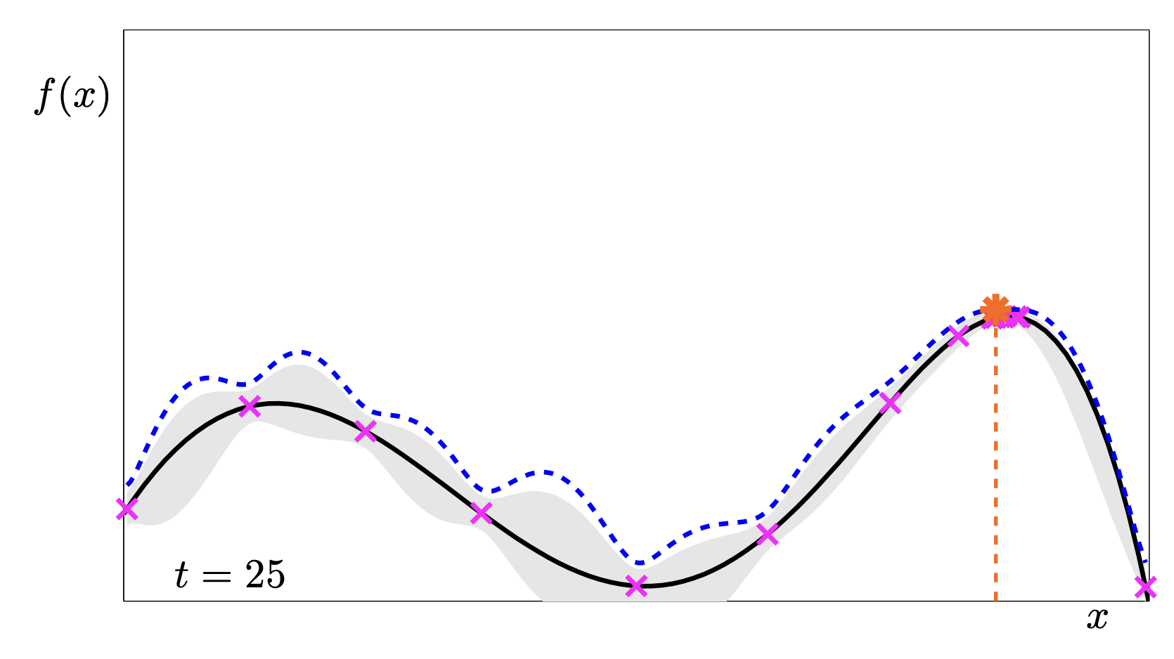
- t=11: We have explored both peaks. The uncertainty is low everywhere relevant. We found the global max.
2.4 Strategy 2 - Thompson Sampling
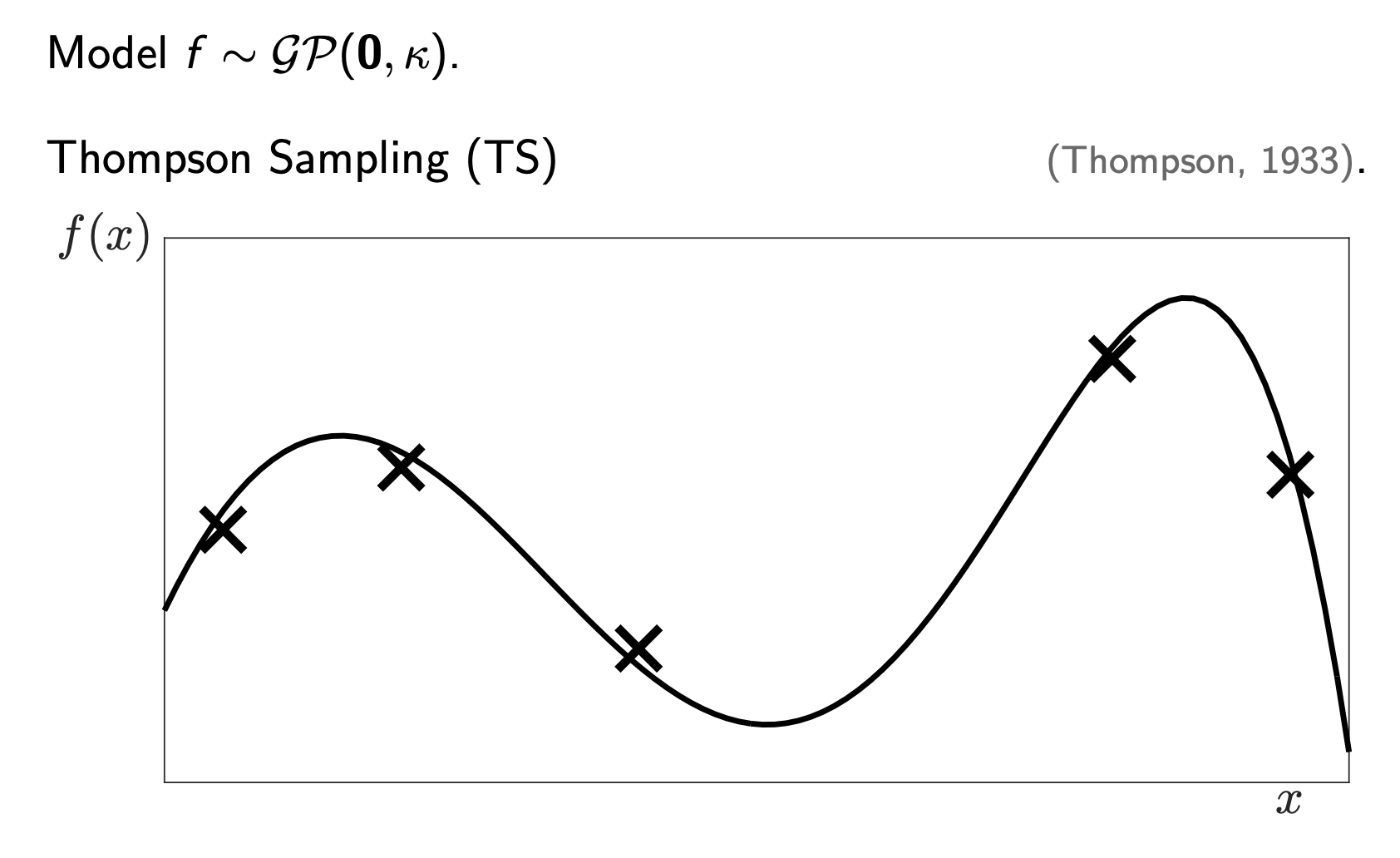
The second strategy is Thompson Sampling (TS) (Thompson 1933). It’s less “algebraic” and more “probabilistic”.
Instead of calculating a specific bound like UCB, we:
- Sample a function \(g(x)\) from the GP posterior. (We roll the dice and generate one possible reality consistent with our data).
- Choose the maximum of that sampled function.
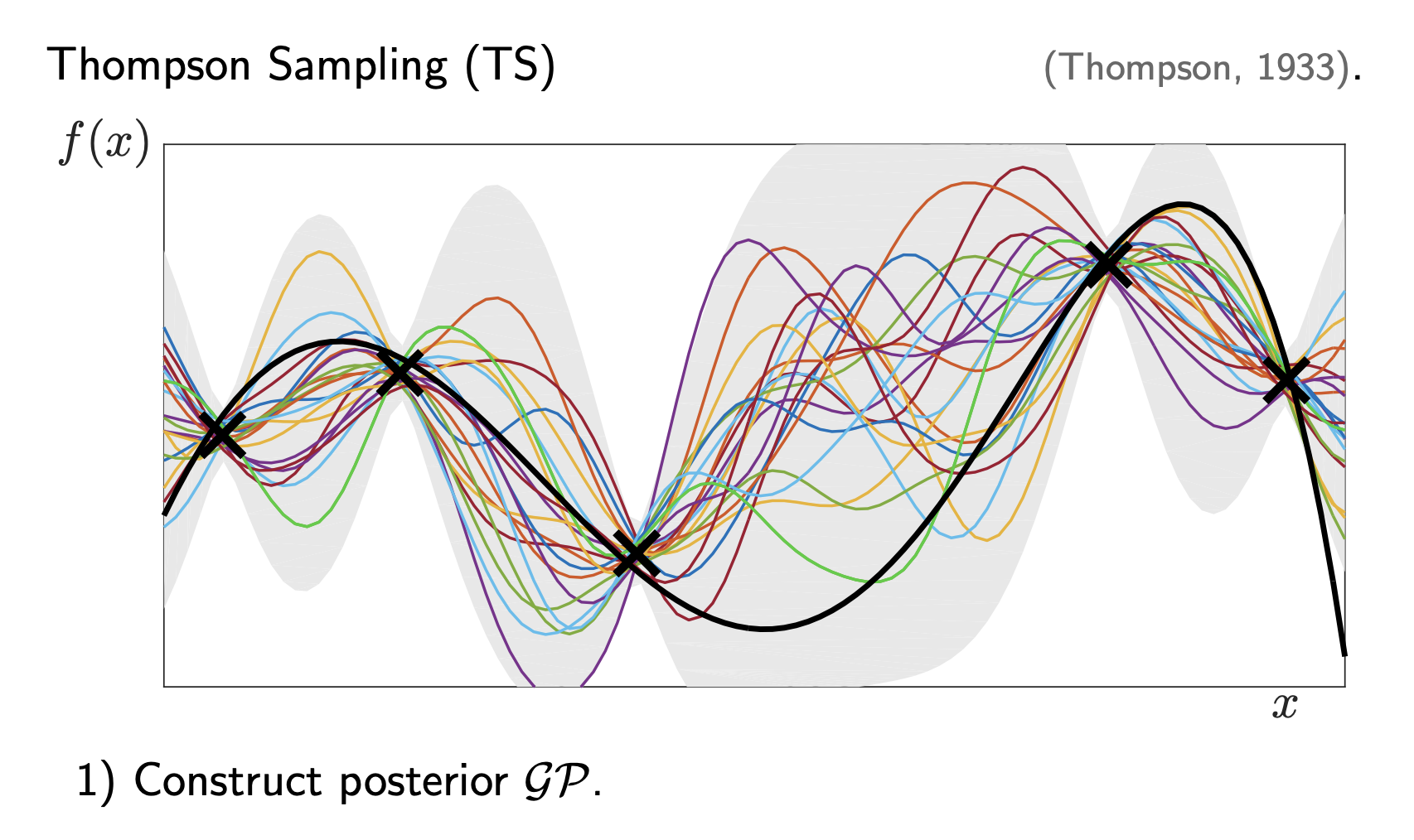
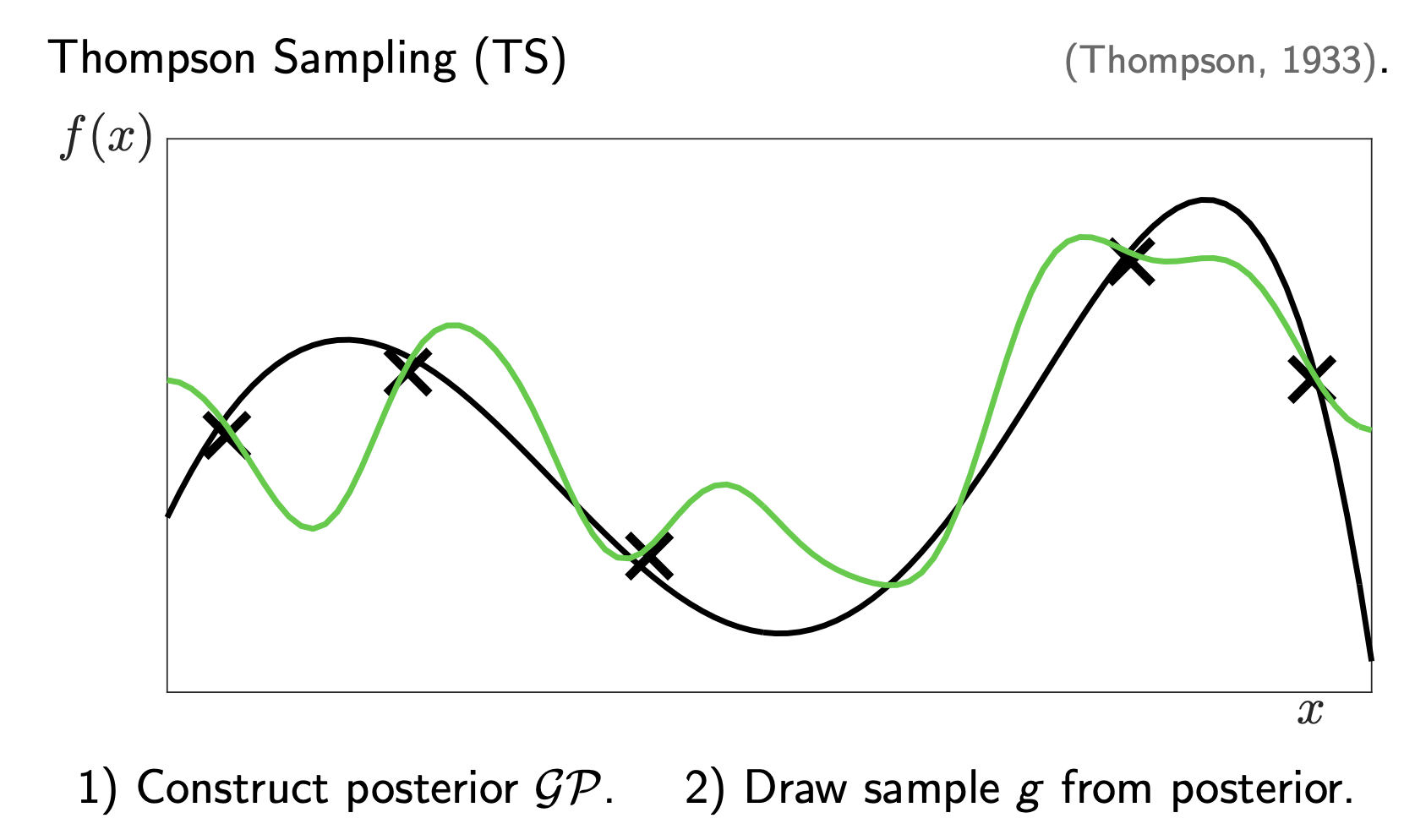
In the second image, the Green Line is one random sample drawn from the GP. Notice how the green line naturally wiggles a lot in the “grey areas” (high variance) but stays close to the mean in the “pinched areas” (low variance).
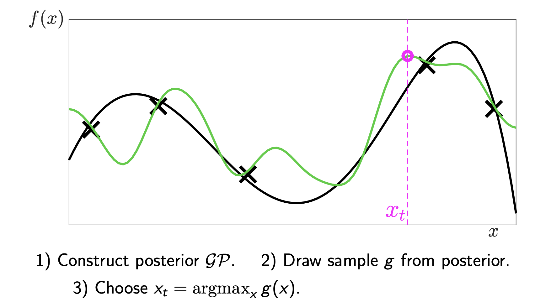
We pick the peak of the green line (the pink circle). This naturally handles the Exploration-Exploitation tradeoff:
- We might sample a function that is high in an uncertain region (Exploration).
- We likely sample a function that is high where the mean is already high (Exploitation).
2.5 Summary: Which to use?
- GP-UCB: Deterministic (given \(\beta\)). Good theoretical guarantees (regret bounds). Explicitly controls the risk.
- Thompson Sampling: Randomized. Often performs better empirically in high dimensions. Easier to implement if you can sample from your model.
Both methods rely on the same “Brain” (the Gaussian Process) to solve the “Expensive Blackbox” problem efficiently.
Next Steps:
If you want to implement this, I highly recommend checking out BoTorch (PyTorch-based) or scikit-optimize. They handle the complex GP math for you!
This post is adapted from (CMU 10-713 F23 2023).